39 how to add data labels to a pie chart in excel on mac
How to Create Pie Charts in Excel (In Easy Steps) Select the pie chart. 9. Click the + button on the right side of the chart and click the check box next to Data Labels. 10. Click the paintbrush icon on the right side of the chart and change the color scheme of the pie chart. Result: 11. Right click the pie chart and click Format Data Labels. 12. Add a Data Callout Label to Charts in Excel 2013 How to Add a Data Callout Label. Click on the data series or chart. In the upper right corner, next to your chart, click the Chart Elements button (plus sign), and then click Data Labels. A right pointing arrow will appear, click on this arrow to view the submenu. Select Data Callout.
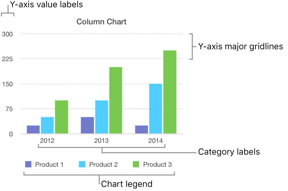
Add column, bar, line, area, pie, donut, and radar charts in Numbers on Mac Create a column, bar, line, area, pie, donut, or radar chart. Click in the toolbar, then click 2D, 3D, or Interactive. Click the left and right arrows to see more styles. Note: The stacked bar, column, and area charts show two or more data series stacked together. Click a chart or drag it to the sheet. If you add a 3D chart, you see at its center.
How to add data labels to a pie chart in excel on mac
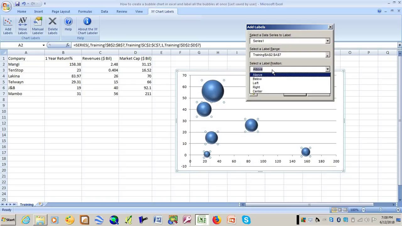
Excel charts: add title, customize chart axis, legend and data labels ... To add a label to one data point, click that data point after selecting the series. Click the Chart Elements button, and select the Data Labels option. For example, this is how we can add labels to one of the data series in our Excel chart: For specific chart types, such as pie chart, you can also choose the labels location. How to Insert Axis Labels In An Excel Chart | Excelchat We will again click on the chart to turn on the Chart Design tab. We will go to Chart Design and select Add Chart Element. Figure 6 - Insert axis labels in Excel. In the drop-down menu, we will click on Axis Titles, and subsequently, select Primary vertical. Figure 7 - Edit vertical axis labels in Excel. Now, we can enter the name we want ... How to Make a PIE Chart in Excel (Easy Step-by-Step Guide) Here are the steps to format the data label from the Design tab: Select the chart. This will make the Design tab available in the ribbon. In the Design tab, click on the Add Chart Element (it's in the Chart Layouts group). Hover the cursor on the Data Labels option.
How to add data labels to a pie chart in excel on mac. Office: Display Data Labels in a Pie Chart 2. If you have not inserted a chart yet, go to the Insert tab on the ribbon, and click the Chart option. 3. In the Chart window, choose the Pie chart option from the list on the left. Next, choose the type of pie chart you want on the right side. 4. Once the chart is inserted into the document, you will notice that there are no data labels. How To Do A Pie Chart In Excel For Mac - bestbup Creatign pie charts from a set of numbers is easy. But if you have to count occurances in a long list of data and create a pie cha. Open Microsoft Excel on your PC or Mac. Open the document containing the data that you'd like to make a pie chart with. Click and drag to highlight all of the cells in the row or column with. Add or remove titles in a chart - support.microsoft.com Show or hide a chart legend or data table Article; Add or remove a secondary axis in a chart in Excel Article; Add a trend or moving average line to a chart Article; Choose your chart using Quick Analysis Article; Update the data in an existing chart Article; Use sparklines to show data trends Article Create a chart in Excel for Mac - support.microsoft.com Click a specific chart type and select the style you want. With the chart selected, click the Chart Design tab to do any of the following: Click Add Chart Element to modify details like the title, labels, and the legend. Click Quick Layout to choose from predefined sets of chart elements.
Broken Y Axis in an Excel Chart - Peltier Tech Nov 18, 2011 · For the many people who do want to create a split y-axis chart in Excel see this example. Jon – I know I won’t persuade you, but my reason for wanting a broken y-axis chart was to show 4 data series in a line chart which represented the weight of four people on a diet. One person was significantly heavier than the other three. How to Make a Pie Chart in Excel — Everything You Need to Know 3. Select the first cell and drag cursor till the last cell to select whole data. 4. Click Insert > Pie. 5. A pie chart will automatically appear. 6. To enter the title of chart, click on highlighted area. 7. Enter your chart's title. Editing Your Pie-Chart Labeling. 1. The labels/values exist as automatically selected. Right-click anywhere ... Change the look of chart text and labels in Numbers on Mac If you can't edit a chart, you may need to unlock it. Change the font, style, and size of chart text Edit the chart title Add and modify chart value labels Add and modify pie chart wedge labels or donut chart segment labels Modify axis labels Edit pivot chart data labels Note: Axis options may be different for scatter and bubble charts. how to convert raw data into column in excel The cell you select becomes the top, left corner of whatever you're copying. Step 2. This opens the Text Import Wizard. Notice how on the attached spreadsheet all of the raw data is in column A under the worksheet "Raw". Open the document containing the data that you'd like to make a pie chart with. Here's where the Data Model magic comes into ...
How to make a pie chart in Excel - ablebits.com To rotate a pie chart in Excel, do the following: Right-click any slice of your pie graph and click Format Data Series. On the Format Data Point pane, under Series Options, drag the Angle of first slice slider away from zero to rotate the pie clockwise. Or, type the number you want directly in the box. Pie Chart in Excel | How to Create Pie Chart - EDUCBA Step 1: Do not select the data; rather, place a cursor outside the data and insert one PIE CHART. Go to the Insert tab and click on a PIE. Step 2: once you click on a 2-D Pie chart, it will insert the blank chart as shown in the below image. Step 3: Right-click on the chart and choose Select Data. Excel Paste And Transpose Shortcut - Automate Excel Paste & Transpose This Excel Shortcut pastes and transposes. PC Shorcut:Ctrl+ALT+V>E>Enter Mac Shorcut:Ctrl+⌘+V>⌘+E>Return Remember This Shortcut: Ctrl + V is the usual command to Paste. Simply add Alt for Paste Special and use E for Transpose. Alernatively you can use Alt > E > S > E . Remember, Alt is the command to activate… How to Create and Format a Pie Chart in Excel - Lifewire To add data labels to a pie chart: Select the plot area of the pie chart. Right-click the chart. Select Add Data Labels . Select Add Data Labels. In this example, the sales for each cookie is added to the slices of the pie chart. Change Colors
30 Create Label In Excel - Label Design Ideas 2020
How To Create A Pie Chart In Excel (With Percentages) - YouTube In this video, I'm going to show you how to create a pie chart by using Microsoft Excel. I will show you how to add data labels that are percentages and even...
How to remove blank rows in Excel to tidy up your sheet - Business Insider
How to Make a Bar Graph in Excel: 9 Steps (with Pictures) May 02, 2022 · Open Microsoft Excel. It resembles a white "X" on a green background. A blank spreadsheet should open automatically, but you can go to File > New > Blank if you need to. If you want to create a graph from pre-existing data, instead double-click the Excel document that contains the data to open it and proceed to the next section.

Format data labels in a chart in Office 2016 for Mac - Office Support
Add a DATA LABEL to ONE POINT on a chart in Excel All the data points will be highlighted. Click again on the single point that you want to add a data label to. Right-click and select ' Add data label '. This is the key step! Right-click again on the data point itself (not the label) and select ' Format data label '. You can now configure the label as required — select the content of ...

New Charts in Excel 2016 • My Online Training Hub
How to Make a Pie Chart in Excel: 10 Steps (with Pictures) If you would rather make a chart from data you already have, double-click the Excel document that contains the data to open it and proceed to the next section. 2 Click Blank workbook (PC) or Excel Workbook (Mac). It's in the top-left side of the "Template" window. 3 Add a name to the chart.
Add a legend, gridlines, and other markings in Pages on Mac - Apple Support
How to show percentage in pie chart in Excel? - ExtendOffice Select the data you will create a pie chart based on, click Insert > I nsert Pie or Doughnut Chart > Pie. See screenshot: 2. Then a pie chart is created. Right click the pie chart and select Add Data Labels from the context menu. 3. Now the corresponding values are displayed in the pie slices.
New Charts in Excel 2016 • My Online Training Hub
How to add percentage to pie chart in excel - kasapwestcoast To add data labels, select the chart and then click on the + button in the top right corner of the pie chart and check the Data Labels button. Initially, the pie chart will not have any data labels in it. Select -> Insert -> Doughnut or Pie Chart -> 2-D Pie. Open Microsoft Excel and select the data that you want to create a pie.

Legend help
Add or remove data labels in a chart - support.microsoft.com Click the data series or chart. To label one data point, after clicking the series, click that data point. In the upper right corner, next to the chart, click Add Chart Element > Data Labels. To change the location, click the arrow, and choose an option. If you want to show your data label inside a text bubble shape, click Data Callout.
Post a Comment for "39 how to add data labels to a pie chart in excel on mac"